Portfolio Optimization

BUSI 721: Data-Driven Finance I

Kerry Back, Rice University

Outline

1. Review of portfolio expected returns and risks
2. Define mean-variance efficient and global minimum variance portfolios
3. Example of quadratic programming with cvxopt
4. SPY, IEF, and GLD returns
5. GMV portfolio of SPY, IEF, and GLD
6. Mean-variance efficient portfolios of SPY, IEF, and GLD
7. Include cash with SPY, IEF, and GLD
8. Sharpe ratios and the tangency portfolio

Review: Portfolio expected return

• With $n$ risky assets,

$$ \sum_{i=1}^n w_i \mu_i + \left(1-\sum_{i=1}^n w_i\right)r_f$$

• where $r_f=$ money market rate if $\sum w_i < 1$ and
• $r_f = $ margin loan rate if $\sum w_i > 1$ and
• we are ignoring interest drag and short borrowing fee if any of the $w_i$ are negative.

Review: Reg T

• Initial margin requirement: when positions are put on,

$$\sum |w_i| \le 2$$

• Afterwards, brokers impose maintenance margin requirements.
• Example: invest 1,000, borrow 1,000, buy 20 shares of $\text{\$}$ 100 stock
  • $\sum w_i = 2$
  • Stock price falls to 75.
  • Now have 1,500 of stock.
  • Portfolio value is 1,500 - 1,000 = 500. Weight on stock is 1,500 / 500 = 3.
  • Maybe get margin call.

Review: Portfolio variance

• Two assets:

$$w_1^2 \sigma_1^2 + w_2^2\sigma_2^2 + 2w_1w_2\rho\sigma_1\sigma_2$$

• Three assets:

$$w_1^2 \sigma_1^2 + w_2^2\sigma_2^2 + w_3^2\sigma_3^2$$$$ + 2w_1w_2\rho_{12}\sigma_1\sigma_2 + 2w_1w_3\rho_{13}\sigma_1\sigma_3 + 2w_2w_3\rho_{23}\sigma_2\sigma_3$$

• Any number of assets:

$$w'\Sigma w$$

Matrix multiplication

$$\begin{pmatrix} a & b\\c & d \end{pmatrix} \begin{pmatrix}x \\y \end{pmatrix} = \begin{pmatrix}ax + by \\cx + dy \end{pmatrix}$$$$\begin{pmatrix} g & h \end{pmatrix} \begin{pmatrix} a & b\\c & d \end{pmatrix} = \begin{pmatrix} ga + hc & gb + hd \end{pmatrix}$$$$\begin{pmatrix} w_1 & w_2 \end{pmatrix} \begin{pmatrix} \sigma_1^2 & \rho_{12}\sigma_1\sigma_2 \\ \rho_{12}\sigma_1\sigma_2 & \sigma_2^2 \end{pmatrix} \begin{pmatrix} w_1 \\ w_2 \end{pmatrix} = \begin{pmatrix} w_1 & w_2 \end{pmatrix} \begin{pmatrix} \sigma_1^2w_1 + \rho\sigma_1\sigma_2 w_2 \\ \rho\sigma_1\sigma_2 w_1 + \sigma_2w_2 \end{pmatrix}$$$$ = \sigma_1^2w_1^2 + \rho\sigma_2\sigma_2w_1w_2 + \rho\sigma_2\sigma_2w_1w_2 + \sigma_2w_2^2$$

2. Mean-Variance Frontier and GMV Portfolio

Mean-Variance Frontier

• Mean-variance frontier is the set of portfolios that have the least risk among all portfolios that have their expected return
• Minimum risk problem: minimize variance subject to constraints:
  • achieve a target expected return
  • $\sum w_i = 1$
  • possibly $w_i \ge 0$ or Reg T
• We can vary the target expected return and trace out the mean-variance frontier
• Some points on the frontier may be inefficient (meaning you can do better on both risk and expected return) because the target expected return is too low.

Global minimum variance portfolio

• Solve the minimization problem without a target expected return
• This portfolio (GMV portfolio) has the least risk among all portfolios
• Frontier portfolios are efficient (meaning you can't do better on both risk and expected return) if and only if the target expected return $\ge $ expected return of GMV portfolio.

3. Quadratic programming

• Finding efficient portfolios and finding the GMV portfolio are examples of quadratic programming
• Minimize or maximize a quadratic function (squares and products and linear terms)
  • Subject to linear inequality constraints
  • And subject to linear equality constraints

Quadratic Programming Example

minimize

$$x_1^2 + x_2^2 - 2x_1 - x_2$$

subject to

$$x_1 \ge 0$$

$$x_2 \ge 0$$ $$x_1+x_2=1$$

Notation of cvxopt

minimize $$\frac{1}{2} x'Px + q'x$$ subject to $$Gx \le h$$ and $$Ax=b$$

Our example

$$P = \begin{pmatrix} 2 & 0 \\ 0 & 2 \end{pmatrix} \quad \Rightarrow \quad \frac{1}{2} x'Px = x_1^2 + x_2^2$$$$ q = \begin{pmatrix} - 2 \\ - 1 \end{pmatrix}\quad\Rightarrow\quad q'x = -2 x_1 - x_2$$$$G =\begin{pmatrix} -1 & 0 \\ 0 & -1 \end{pmatrix}\quad\Rightarrow\quad Gx = \begin{pmatrix} -x_1 \\ -x_2 \end{pmatrix}$$$$h= \begin{pmatrix} 0 \\ 0 \end{pmatrix}$$$$A = \begin{pmatrix} 1 & 1 \end{pmatrix}\quad\Rightarrow\quad Ax = x_1 + x_2$$$$b = \begin{pmatrix} 1 \end{pmatrix}$$

Define arrays

P = np.array(
    [
        [2., 0.],
        [0., 2.]
    ]
)
q = np.array([-2., -1.]).reshape(2, 1)
G = np.array(
    [
        [-1., 0.],
        [0., -1.]
    ]
)
h = np.array([0., 0.]).reshape(2, 1)
A = np.array([1., 1.]).reshape(1, 2)
b = np.array([1.]).reshape(1, 1)

Solve

from cvxopt import matrix
from cvxopt.solvers import qp

sol = qp(
    P=matrix(P),
    q=matrix(q),
    G=matrix(G),
    h=matrix(h),
    A=matrix(A),
    b=matrix(b)
)
np.array(sol["x"])

     pcost       dcost       gap    pres   dres
 0: -1.1111e+00 -2.2222e+00  1e+00  1e-16  1e+00
 1: -1.1231e+00 -1.1680e+00  4e-02  1e-16  4e-02
 2: -1.1250e+00 -1.1261e+00  1e-03  2e-16  3e-04
 3: -1.1250e+00 -1.1250e+00  1e-05  6e-17  3e-06
 4: -1.1250e+00 -1.1250e+00  1e-07  3e-16  3e-08
Optimal solution found.

array([[0.7499999],
       [0.2500001]])

4. Stock, Bond, and Gold ETFs

• SPY, IEF, and GLD adjusted closing prices from Yahoo
• Downsample to monthly
• Percent changes are monthly returns
• Compute historical means and covariance matrix

import yfinance as yf

tickers = ["SPY", "IEF", "GLD"]
prices = yf.download(tickers, start="1970-01-01")["Adj Close"]
prices = prices.resample("M").last()
rets = prices.pct_change().dropna()
rets.head(3)

[*********************100%%**********************]  3 of 3 completed

	GLD	IEF	SPY
Date
2004-12-31	-0.029255	0.011674	0.030121
2005-01-31	-0.036073	0.008710	-0.022421
2005-02-28	0.031028	-0.013683	0.020904

Means, risks and correlations

12 * rets.mean()

GLD    0.087096
IEF    0.031683
SPY    0.100341
dtype: float64

np.sqrt(12) * rets.std()

GLD    0.169435
IEF    0.064872
SPY    0.150749
dtype: float64

rets.corr()

	GLD	IEF	SPY
GLD	1.000000	0.317975	0.084318
IEF	0.317975	1.000000	-0.121379
SPY	0.084318	-0.121379	1.000000

mu = rets.mean().to_numpy()
Sigma = rets.cov().to_numpy()

5. GMV Portfolio of Stocks, Bonds, and Gold

GMV minimization problem

minimize

$$\frac{1}{2} w'\Sigma w$$

subject to

$$\sum w_i = 1 \quad \Leftrightarrow \quad \iota'w = 1$$

where $\iota$ is a column vector of ones.

cvxopt formulation

• $P=\Sigma$
• $q=0$

$$A = \begin{pmatrix} 1 & 1 & 1 \end{pmatrix}$$$$ b = \begin{pmatrix} 1 \end{pmatrix}$$

Define arrays

P = Sigma
q = np.zeros((3, 1))
A = np.ones((1, 3))
b = np.ones((1, 1))

Compute the GMV portfolio

sol = qp(
    P=matrix(P),
    q=matrix(q),
    A=matrix(A),
    b=matrix(b)
)

import pandas as pd
gmv = pd.Series(sol["x"], index=rets.columns)
gmv

GLD   -0.001301
IEF    0.817025
SPY    0.184276
dtype: float64

Risk and expected return of GMV portfolio

w = gmv.to_numpy()
print(f"\nGMV annualized std dev is {np.sqrt(12*w@Sigma@w):.2%}")
print(f"GMV annualized mean is {12*mu@w: .2%}")

print(f"\nIEF annualized std dev is {np.sqrt(12)*rets.IEF.std():.2%}")
print(f"IEF annualized mean is {12*rets.IEF.mean():.2%}")

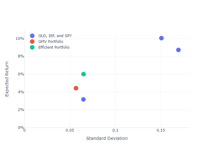
GMV annualized std dev is 5.67%
GMV annualized mean is  4.43%

IEF annualized std dev is 6.49%
IEF annualized mean is 3.17%

6. Efficient portfolios of SPY, IEF, and GLD

Minimize risk with target expected return

minimize

$$\frac{1}{2} w'\Sigma w$$

subject to

$$\mu'w = r$$$$\iota'w = 1$$

where $r=$ target expected return and $\iota$ is a column vector of ones.

cvxopt formulation

• $P=\Sigma$
• $q=0$

$$A = \begin{pmatrix} \mu_1 & \mu_2 & \mu_3 \\ 1 & 1 & 1 \end{pmatrix}$$$$ b = \begin{pmatrix} r \\ 1 \end{pmatrix}$$

Define arrays

# example target monthly expected return
r = 0.06/12

P = Sigma
q = np.zeros((3, 1))
A = np.array(
    [
        mu,
        [1., 1., 1.]
    ]
)
b = np.array([r, 1]).reshape(2, 1)

Compute the efficient portfolio

sol = qp(
    P=matrix(P),
    q=matrix(q),
    A=matrix(A),
    b=matrix(b)
)
efficient = pd.Series(sol["x"], index=rets.columns)
efficient

GLD    0.115466
IEF    0.565289
SPY    0.319245
dtype: float64

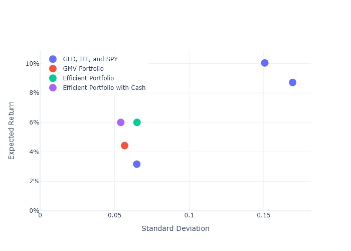
7. Include cash with SPY, IEF, and GLD

Target expected return with cash

• Expected return is

$$\mu'w + (1-\iota'w)r_f = r_f + (\mu-r_f\iota')w$$

• Equals target expected return $r$ if and only if

$$(\mu-r_f\iota)'w = r-r_f$$

• So,

$$A = \begin{pmatrix} \mu_1-r_f & \mu_2-r_f & \mu_3-r_f \end{pmatrix}$$$$b = \begin{pmatrix} r-r_f \end{pmatrix}$$

Define arrays

# example monthly interest rate
rf = 0.03/12

# example target expected return
r = 0.06/12

P = Sigma
q = np.zeros((3, 1))
A = (mu - rf*np.ones(3)).reshape(1, 3)
b = np.array([r-rf]).reshape(1, 1)

Compute the efficient portfolio

sol = qp(
    P=matrix(P),
    q=matrix(q),
    A=matrix(A),
    b=matrix(b)
)
efficient_with_cash = pd.Series(sol["x"], index=rets.columns)
efficient_with_cash

GLD    0.176189
IEF   -0.027139
SPY    0.284129
dtype: float64

8. Sharpe Ratios and the Tangency Portfolio

Sharpe ratio

• The Sharpe ratio is defined as

$$\frac{\text{Expected Return} - \text{Risk-Free Rate}}{\text{Standard Deviation}}$$

• To annualize a monthly Sharpe ratio,
  • numerator should be multiplied by $12$,
  • denominator should be multiplied by $\sqrt{12}$
  • so ratio should be multiplied by $\sqrt{12}$

Sharpe ratios of SPY, IEF, and GLD

sharpes = np.sqrt(12)*(rets.mean() - rf) / rets.std()
sharpe_efficient = np.sqrt(12)*(r - rf) / np.sqrt(w@Sigma@w)

print(f"SPY = {sharpes.SPY:.2%}")
print(f"IEF = {sharpes.IEF:.2%}")
print(f"GLD = {sharpes.GLD:.2%}")
print(f"Efficient portfolio with cash = {sharpe_efficient:.2%}")

SPY = 46.66%
IEF = 2.59%
GLD = 33.70%
Efficient portfolio with cash = 55.43%

Geometry of Sharpe ratios

• Sharpe ratio is slope of line connecting (std dev=0, mean=rf) with the (std dev, mean) of the asset or portfolio
• Efficient portfolios with cash all have the same Sharpe ratio, so they all lie on the same line
• This is the maximum possible Sharpe ratio - the line is the furthest northwest in the (std dev, mean) diagram.

Tangency portfolio

• Tangency portfolio is an efficient portfolio with cash that does not use cash
• It is efficient with or without cash
• It is the point at which the line with maximum Sharpe ratio just touches the frontier without cash
• We should hold the tangency portfolio with or without cash
• Will look at margin loans later

Tangency portfolio of SPY, IEF, and GLD

tang = w / np.sum(w)
pd.Series(tang, index=rets.columns).round(3)

GLD    0.407
IEF   -0.063
SPY    0.656
dtype: float64